
Analysis and Predict the Volatility of Nasdaq-100 through Machine Learning
1. Abstract
The Nasdaq-100, a benchmark index dominated by high-growth technology firms, exhibits distinct volatility patterns that reflect inherent financial risks. This study investigates the historical volatility trends and employs predictive models—GARCH, Random Forest, and Neural Network Auto-Regressive (NNAR)—to forecast future volatility. Historical volatility is quantified as the rolling standard deviation of log returns over a 30-day window, leveraging data from 2010 to 2024. While GARCH remains a robust traditional model for capturing heteroscedasticity, machine learning methods like Random Forest and NNAR offer insights into non-linear patterns and feature interactions. The result indicates that the volatility of Nasdaq-100 is going to be increase in the short term, according to the result prediction of Random Forest, as its lowest RMSE, which means the probability of its precise prediction is higher that others. It highlight the trade-offs in predictive accuracy and computational efficiency among these models, providing a comprehensive approach for investors and analysts in risk management and strategic decision-making. This study underscores the importance of combining traditional and modern techniques for robust volatility forecasting.
2. Introduction and Objective
The volatility of a time series is calculated by standard deviation or variance, otherwise, of the expected errors (Hang, N. T., & Nam, V. Q. 2021), here, will be defined as the standard deviation of log returns over a given rolling window (e.g., 30 days). Predicting volatility is crucial for risk management, options pricing, and strategic asset allocation.
Investors and traders require not only predictions of future returns but also estimations of associated risks to optimize their decision-making processes. Volatility, reflecting the risk factor of financial time series, is a measure of uncertainty or variability around the expected value. It is often characterized by features such as heteroscedasticity and volatility clustering, which show periods of high and low volatility occurring in sequences.
The Nasdaq 100 is known for its high volatility due to its composition of high-growth, technology-focused companies. This report is aims to:
Analyse historical volatility trends.
Predict future volatility using machine learning models.
Compare the performance of different machine learning methods to identify the most suitable approach for this task.
Definition of Volatility
Historical volatility can be computed as the standard deviation of daily log returns over a chosen window. For example, a 30-day rolling standard deviation of returns.
Why Machine Learning?
Traditional financial models, such as GARCH (Generalized Auto-Regressive Conditional Heteroscedasticity), have been widely used for volatility prediction. Financial time series often exhibit volatility clustering due to heteroscedaticity, making classical time series model like GARCH highly suitable for predicting future volatility, as they assume stationarity but account for time-varying conditional variance. However, they rely on strong parametric assumptions. Recently, machine learning techniques, such as decision trees (Brunello, A., et al 2019) and neural network models (including NNAR-Neural Network Auto-Regressive), have provided additional methods for forecasting volatility by leveraging past values to predict future outcomes. Machine learning models can potentially capture complex non-linear relationships and incorporate a broader set of features (e.g., technical indicators, macroeconomic variables).
GARCH is a popular stochastic model for forecasting time series volatility, extending ARCH by allowing conditional variance to depend on previous errors and volatility (Bollerslev, T. 1986). By capturing volatility clustering, it effectively models financial series like stock prices, exchange rates, and inflation rates (McNees, S. 1973; Tsay, R. S. 2005), although its stationarity assumption requires a time-invariant mean and variance (Tsay, R. S. 2005; Satchell, S., & Knight, J. 2011). GARCH often outperforms in short-term forecasts because predictions converge toward the unconditional variance (Hamilton 1994), and empirical studies support its usefulness for volatile financial indices (Kanasro, H. A., et al. 2009; Fakhfekh, M., & Jeribi, A. 2020). However, the model assumes symmetric responses to positive and negative shocks, which is not always realistic. In parallel, artificial neural networks (ANNs), which mimic human brain function, excel at extracting complex patterns from data (Basheer, I. A., & Hajmeer, M. 2000; Maleki, A. et al. 2018). Models like NNAR (Neural Network Auto-Regressive) leverage lagged values to predict future outcomes and have shown promise in stock price forecasting (Khan, M. A., et al. 2017), though comparisons suggest that for certain short-term predictions, conventional statistical models can still perform better (Islam, M. R., & Nguyen, N. 2020).
We will use R1, as it is well-suited for statistical and financial analysis. The methods include:
GARCH (Generalized Auto-Regressive Conditional Heteroscedasticity)
Random forest
Neural Network Auto-Regressive (NNAR)
3. Data Collection and Preprocessing
Data Source:
Use quantmod package to get the historical price data from the Nasdaq-100 index from 2010-01-01 to 2024-12-20. Calculate daily log returns, which is presented in Figure 1 to compute historical volatility (our target variable) as the rolling standard deviation of log returns.
Daily log returns are calculated using:

The formula for calculating the rolling standard deviation to measure historical volatility is as follows:

Fig 1. Daily Log Returns & 30-Day Rolling Historical volatility of Nasdaq-100
The historical volatility analysis reveals distinct periods of volatility clustering, where high and low volatility phases occur in succession, consistent with financial time series' heteroscedastic nature. Spikes in volatility align with major market events, indicating increased uncertainty and risk during those times, while prolonged periods of low volatility reflect market stability. The rolling window approach effectively captures short-term variability without overreacting to anomalies, providing a smoothed perspective of volatility trends. The training period (2010–2020) includes diverse market conditions, ensuring a robust foundation for model training, while the test period (2021–2024) reflects recent dynamics, testing the adaptability of predictive models. These observations underscore the need for models capable of handling non-stationary, time-dependent relationships, validating the use of GARCH, Random Forest, and Neural Network Auto-Regressive methods for forecasting.
4. Baseline Models (Historical Measures and GARCH)
The GARCH (Generalized Autoregressive Conditional Heteroskedasticity) model, introduced by Bollerslev (1986), is an extension of the ARCH model designed to model and forecast time-series volatility. It is particularly effective for financial time series that exhibit volatility clustering, where periods of high and low volatility occur consecutively. Unlike the ARCH model, which only accounts for past squared residuals, GARCH incorporates both past squared residuals and lagged conditional variances, making it a more comprehensive model for capturing heteroskedasticity. The underlying assumption of stationarity ensures that the time series has time-invariant mean and variance, while the conditional variance evolves dynamically based on historical data.
The GARCH(1,1) model, one of the simplest forms, is expressed as:

Fig 2. Nasdaq-100 Actual vs. Predicted Volatility (GARCH)
5. Machine Learning Methods
Random Forest model
The Random Forest model, introduced by Breiman (2001), is an ensemble learning method that combines multiple decision trees to enhance predictive accuracy and reduce overfitting. It operates by constructing a collection of decision trees during training and outputting either the mode of the classifications (for classification tasks) or the mean prediction (for regression tasks) of the individual trees. Each tree is built using a bootstrap sample of the data, and at each split, a random subset of features is considered, which introduces diversity among the trees and improves generalization. This method is robust to overfitting and works well with high-dimensional data and non-linear relationships.

Bootstrapping: Each tree is trained on a randomly sampled subset (with replacement)
of the original data.
Feature Subsetting: At each split in a tree, a random subset of features is chosen for consideration, enhancing the model's ability to handle high-dimensional data.
Random Forest is robust to overfitting because it averages predictions across many trees, reducing variance. It handles both regression and classification tasks effectively. Randomization in data sampling and feature selection ensures diverse decision boundaries and improved model stability. The result of employing the Random Forest to predict the volatility of Nasdaq-100 is shown in Figure 3, which indicating the upward trend of its volatility in the short term.
Fig 3. Nasdaq-100 Volatility Prediction: In-Sample and Out-of-Sample (Random Forest)
6. Neural Network Auto-Regressive (NNAR)
The Neural Network Auto-Regressive (NNAR) model is a feed-forward neural network approach designed specifically for time-series forecasting. It extends traditional autoregressive (AR) models by incorporating non-linear transformations using a neural network architecture. The NNAR model uses lagged values of the time series as inputs and employs a network structure with three layers: input, hidden, and output (Maleki, A., Nasseri, S., Aminabad, M. S., & Hadi, M., 2018). It is particularly effective for handling non-linear relationships and autoregressive structures in time-series data. The model adapts well to data without explicit seasonality, making it suitable for various forecasting tasks.

The NNAR captures non-linear patterns in the data. It uses lagged values as inputs, like traditional AR models and performs well without explicit seasonal components, although it can handle them when included. The result of employing the NNAR to predict the volatility of Nasdaq-100 is shown in Figure 4, which indicating that its volatility may be going to decline in the short run.
Fig 4. Nasdaq-100 Volatility Prediction: In-Sample and Out-of-Sample (NNAR)
7. Conclusion
Below is one possible way to compare all four models (GARCH(1,1), GJR-GARCH, Random Forest, and NNAR) on the same plot and calculate basic error metrics (e.g., MSE, RMSE) for the in-sample test period, which is shown in Figure 5. The result indicates that the volatility of Nasdaq-100 is going to be increase, according to the result prediction of Random Forest, as its lowest RMSE,which means the probability of its precise prediction is higher that others.
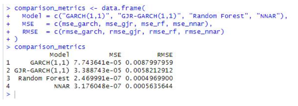
Fig 5. The Comparison Metrics of different method used to predict the volatility of Nasdaq-100
This analysis provides a comprehensive evaluation of GARCH, Random Forest, and NNAR models in forecasting the volatility of the Nasdaq-100. GARCH demonstrated strong short-term forecasting capabilities, accurately capturing volatility clustering and time-varying conditional variance. However, its reliance on stationarity assumptions and inability to handle asymmetric shocks or complex non-linearities limit its applicability in highly dynamic markets. Random Forest, by leveraging ensemble learning and feature subsetting, showed robustness in capturing non-linear patterns and performing well under diverse market conditions. Nevertheless, it struggled with overfitting to noise when feature selection was not carefully managed and required significant computational time for large datasets. NNAR excelled in capturing intricate, non-linear relationships but was computationally intensive and prone to overfitting in the absence of careful parameter tuning, particularly for smaller training datasets.
The comparative analysis highlights that while each method offers distinct strengths — GARCH for interpretability, Random Forest for robustness, and NNAR for precision — none is without limitations. To overcome these challenges, hybrid frameworks combining the strengths of these models may provide more reliable and accurate forecasts. Future work should explore integrating additional data sources, such as macroeconomic indicators or market sentiment, and develop ensemble methods that mitigate individual model weaknesses. These insights contribute to informed decision-making in risk management, strategic asset allocation, and options pricing, while acknowledging the inherent trade-offs of each predictive approach.
-
We are grateful for Prof. Deep Kapur and the team at Monash Centre for Financial Studies (MCFS) for their unwavering support on a student-led initiative and the delivery of our agenda in multiple of ways and acknowledge their contributions to each and all releases. We also remain deeply grateful to the Faculty of Banking and Finance at Monash Business School for continuous support in facilitation of MSMF and our agenda.
-
This material is a product of Monash Student Managed Fund (MSMF) and is provided to you solely for general information purposes. I understand that the information in these documents is NOT financial advice. Before making an investment decision to acquire shares, you should consider, preferably with the assistance of a financial or other professional adviser, whether an investment is appropriate in light of your own personal circumstances. If you can, you should obtain a copy of the Information Memorandum of the company that you are seeking to invest in, and consider their risks and disclosures. Subject to the Australian Consumer Law, Corporations Act, the ASIC Act, and any other relevant law, MSMF does not accept any responsibility for any loss to any person incurred as a result of reliance on the information, including any negligent errors or omissions. This information is strictly the personal opinion of an MSMF member and does not represent the views of MSMF. This information constitutes factual information that is objectively ascertainable such that the truth or accuracy of which cannot reasonably be questioned. MSMF does not intend to advertise any stock or financial product whatsoever. Past performance is not a reliable indicator of future performance. Past asset allocation and gearing levels may not be reliable indicators of future asset allocation and gearing levels. Performance data is just an estimation based on public market data and may not be a true reflection of actual fund performance.
-
Basheer, I., & Hajmeer, M. (2000). Artificial neural networks: Fundamentals, computing, design, and application. Journal of Microbiological Methods, 43(1), 3-31.
Bollerslev, T. (1986). Generalized autoregressive conditional heteroskedasticity. Journal of econometrics, 31(3), 307-327.
Breiman, L. (2001). Random forests. Machine Learning, 45(1), 5–32.
Brunello, A., Marzano,E., Montanari, A., & Sciavicco, G. (2019). J48SS: Anovel decision tree approach for the handling of sequential and time series data. Computers, 8(1), 21.
Hamilton, J.D (1994). Time Series Analysis 2 Princeton: Princeton University Press.
Hang, N. T., & Nam, V. Q. (2021). Formulation Of Beta Capm Index With Weighted Average Methods And Market Risk Comparison Of Listed Banks During PostGlobal Crisis Period 2011-2020.
Islam, M. R., & Nguyen, N. (2020). Comparison of financial models for stock price prediction. Journal of Risk and Financial Management, 13(8), 181.
Kanasro, H. A., Rohra, C. L., & Junejo, M. A. (2009). Measurement of stock market volatility through ARCH and GARCH models: a case study of Karachi stock exchange. Australian Journal of Basic and Applied Sciences, 3(4), 3123-3127.
Khan, M. A., Khan, N., Hussain, J., Shah,N. H., & Abbas, Q. (2017). Validity of technical analysis indicators: A case of KSE-100 index. Abasyn University Journal of Social Sciences, 10(1), 1-19.
Maleki, A., Nasseri, S., Aminabad, M. S., & Hadi, M. (2018). Comparison of ARIMA and NNAR models for forecasting water treatment plant’s influent characteristics. KSCE Journal of Civil Engineering, 22(9), 3233–3245.
McNees, S.S. (1973) The Forecasting Record for the 1970s, New England Economic Review.
RColorBrewer, S., & Liaw, M. A. (2018). Package “randomforest’’. Berkeley, CA, USA: University of California, Berkeley.
Tsay, R. S. (2005). Analysis of financial time series. Wiley Series in Probability and Statistics.

Author
Kaidong Zeng- Research Associate
Kaidong Zeng is currently a Research Associate in MSMF Institute (Australian Desk), and is currently pursuing a Masters in Business Economics.